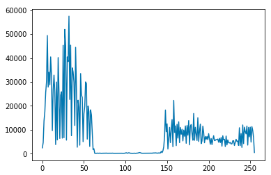
ヒストグラム
ヒストグラムを用いることで、解析したい画像の中にどの色(青など)が多いのか調べることができます。
正確に言えば、画素値の分布を描画することで視覚的に分かりやすくします。
import cv2
import matplotlib.pyplot as plt
%matplotlib inline

# 画像の確認
img  = cv2.imread('sample.png')

cv2.imshow('img', img)

cv2.waitKey(0) & 0xFF
cv2.destroyAllWindows()
cv2.waitKey(1) & 0xFF

# RGBのヒストグラム
color_list = ['blue', 'green', 'red']
for i, j in enumerate(color_list):
    hist = cv2.calcHist([img], [i], None, [256], [0, 256])
    plt.plot(hist, color=j)

# グレースケールのヒストグラム
img_gray = cv2.imread('sample.png', 0)
hist2  = cv2.calcHist([img_gray], [0], None, [256], [0, 256])
plt.plot(hist2)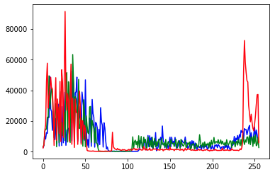
ヒストグラム平坦化
平坦化は均一化や均等化などとも呼ばれたりしますが、全部同じ意味と思っていただいて大丈夫です。
平坦化を行うと、画像のコントラストが強調されて、見たい画像の箇所をはっきりと見ることが可能になります。
注意点としては、カラー画像には使えないので、グレースケール化は必須です。
import cv2
import matplotlib.pyplot as plt
%matplotlib inline
img = cv2.imread('sample.png', 0)
hist = cv2.calcHist([img], [0], None, [256], [0, 256])
plt.plot(hist)
img_eq = cv2.equalizeHist(img)
hist_e = cv2.calcHist([img_eq], [0], None, [256], [0, 256])
plt.plot(hist_e)
# 平坦化とオリジナル画像の比較
cv2.imshow('img', img)
cv2.imshow('eq', img_eq)
cv2.waitKey(0) & 0xFF
cv2.destroyAllWindows()
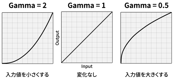
cv2.waitKey(1) & 0xFFγ(ガンマ)変換
γ(ガンマ)変換とは画像の明るさの変換方法です。
γが1の場合は直線になり、入力と出力が同じになります。
γが1未満の場合には画像が暗くなり、逆に1を超えると明るくなります。
import cv2
import numpy as np

gamma = 1.5
img = cv2.imread('Lenna_(test_image).png')
gamma_cvt = np.zeros((256, 1), dtype=np.uint8)
for i in range(256):
    gamma_cvt[i][0] = 255 * (float(i)/255) ** (1.0 / gamma)

img_gamma = cv2.LUT(img, gamma_cvt)

cv2.imshow('img', img)
cv2.imshow('gamma', img_gamma)

cv2.waitKey(0) & 0xFF
cv2.destroyAllWindows()
cv2.waitKey(1) & 0xFF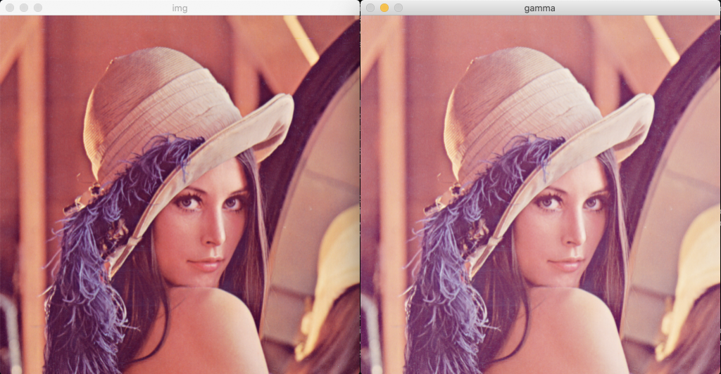
補足
トラックバーの作成
import cv2

def onTrackbar(position):
    global trackValue
    trackValue = position # 表示位置

trackValue = 100
cv2.namedWindow('img')
cv2.createTrackbar('track', 'img', trackValue, 255, onTrackbar)

img = cv2.imread('Lenna_(test_image).png')
cv2.imshow('img', img)

cv2.waitKey(0) & 0xFF
cv2.destroyAllWindows()
cv2.waitKey(1) & 0xFF
マウスイベント
import cv2
import numpy as np

def print_position(event, x, y, flags, param):
    if event == cv2.EVENT_LBUTTONDOWN: # クリックされたら
        print(x, y) # 座標表示


img = np.zeros((512, 512), np.uint8)
cv2.namedWindow('img')
cv2.setMouseCallback('img', print_position)
cv2.imshow('img', img)

cv2.waitKey(0) & 0xFF
cv2.destroyAllWindows()
cv2.waitKey(1) & 0xFF
2値化
閾値の取り方は、手動で設定するやり方や、分布を見て自動的に設定してくれるやり方だなどが存在します。
import cv2
import matplotlib.pyplot as plt
%matplotlib inline

img = cv2.imread('Lenna_(test_image).png', 0)
threshold  = 100 # 閾値
ret, img_th = cv2.threshold(img, threshold, 255, cv2.THRESH_BINARY)

cv2.imshow('img_th', img_th)
cv2.waitKey(0) & 0xFF
cv2.destroyAllWindows()
cv2.waitKey(1) & 0xFF

hist = cv2.calcHist([img], [0], None, [256], [0, 256])
plt.plot(hist)

ret2, img_o = cv2.threshold(img, 0, 255, cv2.THRESH_OTSU)

cv2.imshow('img_o', img_o)
cv2.waitKey(0) & 0xFF
cv2.destroyAllWindows()
cv2.waitKey(1) & 0xFF
2値化とトラックバーの組み合わせ
import cv2

img = cv2.imread('Lenna_(test_image).png', 0)

def onTrackbar(position):
    global threshold
    threshold = position
    ret, img_th = cv2.threshold(img, threshold, 255, cv2.THRESH_BINARY)
    # img_th = cv2.adaptiveThreshold(img, 255, cv2.ADAPTIVE_THRESH_MEAN_C, cv2.THRESH_BINARY, 3, threshold)
    cv2.imshow('img', img_th)

cv2.namedWindow('img')
threshold = 100
cv2.createTrackbar('track', 'img', threshold, 255, onTrackbar)
while True:
    ret, img_th = cv2.threshold(img, threshold, 255, cv2.THRESH_BINARY)
    cv2.imshow('img', img_th)
    if cv2.waitKey(10) & 0xFF:
        break

cv2.waitKey(0) & 0xFF
cv2.destroyAllWindows()
cv2.waitKey(1) & 0xFF